A Guide to Working with Quantities

Introduction

This document intends to be a guide on how to work with quantities data (magnitudes with units and/or uncertainty) in two distinct workflows: R base and the so-called tidyverse. Units and errors (and, by extension, quantities) objects essentially are numeric vectors, arrays and matrices with associated metadata. This metadata is not always compatible with some functions, and thus we here explore the most common operations in data wrangling (subsetting, ordering, transformations, aggregations…) to identify potential issues and propose possible workarounds.

Let us consider the traditional iris data set for this exercise. According to its documentation,

iris is a data frame with 150 cases (rows) and 5 variables (columns) named Sepal.Length, Sepal.Width, Petal.Length, Petal.Width, and Species.

And values are provided in centimeters. If we consider, for instance, a 2% of uncertainty, the first step is to define proper quantities. Then we will work on the resulting data frame for the rest of this article.

library(quantities)
#> Loading required package: units
#> udunits database from /usr/share/xml/udunits/udunits2.xml
#> Loading required package: errors

iris.q <- iris
for (i in 1:4)
  quantities(iris.q[,i]) <- list("cm", iris.q[,i] * 0.02)
head(iris.q)
#>   Sepal.Length  Sepal.Width Petal.Length   Petal.Width Species
#> 1  5.1(1) [cm] 3.50(7) [cm] 1.40(3) [cm] 0.200(4) [cm]  setosa
#> 2  4.9(1) [cm] 3.00(6) [cm] 1.40(3) [cm] 0.200(4) [cm]  setosa
#> 3 4.70(9) [cm] 3.20(6) [cm] 1.30(3) [cm] 0.200(4) [cm]  setosa
#> 4 4.60(9) [cm] 3.10(6) [cm] 1.50(3) [cm] 0.200(4) [cm]  setosa
#> 5  5.0(1) [cm] 3.60(7) [cm] 1.40(3) [cm] 0.200(4) [cm]  setosa
#> 6  5.4(1) [cm] 3.90(8) [cm] 1.70(3) [cm] 0.400(8) [cm]  setosa

Note that, throughout this document, and unless otherwise stated, we will talk about quantities objects as a shortcut for quantities, units and errors objects.

R Base

In this section, we consider all the methods and functions included in the default packages, i.e., those that are automatically installed along with any R distribution:

rownames(installed.packages(priority="base"))

#>  [1] "base"      "compiler"  "datasets"  "graphics"  "grDevices" "grid"     
#>  [7] "methods"   "parallel"  "splines"   "stats"     "stats4"    "tcltk"    
#> [13] "tools"     "utils"

Row Subsetting

Quantities objects have all the subsetting methods defined ([, [[, [<-, [[<-). Therefore they can be used in the same way as with plain numeric vectors, and in conjunction with which and other functions to perform subsetting. The subset function is very handy too and achieves the same result:

iris.q[which(iris.q$Sepal.Length > set_quantities(75, mm)), ]
#> Warning: In '>' : boolean operators not defined for 'errors' objects,
#> uncertainty dropped
#>     Sepal.Length  Sepal.Width Petal.Length  Petal.Width   Species
#> 106  7.6(2) [cm] 3.00(6) [cm]  6.6(1) [cm] 2.10(4) [cm] virginica
#> 118  7.7(2) [cm] 3.80(8) [cm]  6.7(1) [cm] 2.20(4) [cm] virginica
#> 119  7.7(2) [cm] 2.60(5) [cm]  6.9(1) [cm] 2.30(5) [cm] virginica
#> 123  7.7(2) [cm] 2.80(6) [cm]  6.7(1) [cm] 2.00(4) [cm] virginica
#> 132  7.9(2) [cm] 3.80(8) [cm]  6.4(1) [cm] 2.00(4) [cm] virginica
#> 136  7.7(2) [cm] 3.00(6) [cm]  6.1(1) [cm] 2.30(5) [cm] virginica
subset(iris.q, Sepal.Length > set_quantities(75, mm))
#>     Sepal.Length  Sepal.Width Petal.Length  Petal.Width   Species
#> 106  7.6(2) [cm] 3.00(6) [cm]  6.6(1) [cm] 2.10(4) [cm] virginica
#> 118  7.7(2) [cm] 3.80(8) [cm]  6.7(1) [cm] 2.20(4) [cm] virginica
#> 119  7.7(2) [cm] 2.60(5) [cm]  6.9(1) [cm] 2.30(5) [cm] virginica
#> 123  7.7(2) [cm] 2.80(6) [cm]  6.7(1) [cm] 2.00(4) [cm] virginica
#> 132  7.9(2) [cm] 3.80(8) [cm]  6.4(1) [cm] 2.00(4) [cm] virginica
#> 136  7.7(2) [cm] 3.00(6) [cm]  6.1(1) [cm] 2.30(5) [cm] virginica

Note that another quantities object is defined for the comparison. This is needed because different units are incomparable. Also note that the first line throws a warning telling us that the uncertainty was dropped for this operation. This kind of warning is thrown once, and this is why subset succeeds silently.

Row Ordering

The sort function, as its name suggests, sorts vectors, and it is compatible with quantities:

iris.q$Sepal.Length[1:5]
#> Units: [cm]
#> Errors: 0.102 0.098 0.094 0.092 0.100
#> [1] 5.1 4.9 4.7 4.6 5.0
sort(iris.q$Sepal.Length[1:5])
#> Units: [cm]
#> Errors: 0.092 0.094 0.098 0.100 0.102
#> [1] 4.6 4.7 4.9 5.0 5.1

More generally, the order function can be used for data frame ordering:

head(iris.q[order(iris.q$Sepal.Length), ])
#>    Sepal.Length  Sepal.Width Petal.Length   Petal.Width Species
#> 14 4.30(9) [cm] 3.00(6) [cm] 1.10(2) [cm] 0.100(2) [cm]  setosa
#> 9  4.40(9) [cm] 2.90(6) [cm] 1.40(3) [cm] 0.200(4) [cm]  setosa
#> 39 4.40(9) [cm] 3.00(6) [cm] 1.30(3) [cm] 0.200(4) [cm]  setosa
#> 43 4.40(9) [cm] 3.20(6) [cm] 1.30(3) [cm] 0.200(4) [cm]  setosa
#> 42 4.50(9) [cm] 2.30(5) [cm] 1.30(3) [cm] 0.300(6) [cm]  setosa
#> 4  4.60(9) [cm] 3.10(6) [cm] 1.50(3) [cm] 0.200(4) [cm]  setosa

Column Transformation

The transform function is able to modify variables in a data frame or to create new ones. The within function provides a similar but more flexible approach though. Both are fully compatible with quantities:

head(within(iris.q, {
  Sepal.Area <- Sepal.Length * Sepal.Width
  Petal.Area <- Petal.Length * Petal.Width
  rm(Sepal.Length, Sepal.Width, Petal.Length, Petal.Width)
}))
#>   Species      Petal.Area     Sepal.Area
#> 1  setosa 0.280(8) [cm^2] 17.8(5) [cm^2]
#> 2  setosa 0.280(8) [cm^2] 14.7(4) [cm^2]
#> 3  setosa 0.260(7) [cm^2] 15.0(4) [cm^2]
#> 4  setosa 0.300(8) [cm^2] 14.3(4) [cm^2]
#> 5  setosa 0.280(8) [cm^2] 18.0(5) [cm^2]
#> 6  setosa  0.68(2) [cm^2] 21.1(6) [cm^2]

Row Aggregation

Row aggregation is the process of summarising data based on some grouping variable(s). There are several ways of working with data split by factors in R base, and, although they tend to preserve classes, they are generally not very kind to other metadata (i.e., attributes) by default.

In the following example, the average Sepal.Length is computed per Species, but the metadata gets dropped:

tapply(iris.q$Sepal.Length, iris.q$Species, mean)
#>     setosa versicolor  virginica 
#>      5.006      5.936      6.588

Many of these functions include a simplify parameter which, if set to FALSE, preserves quantities metadata:

(sepal.length.agg <- 
   tapply(iris.q$Sepal.Length, iris.q$Species, mean, simplify=FALSE))
#> $setosa
#> 5.0(1) [cm]
#> 
#> $versicolor
#> 5.9(1) [cm]
#> 
#> $virginica
#> 6.6(1) [cm]

The only drawback is that the result is a list, and such a list must be unlisted with care, otherwise, metadata gets dropped again:

# drops quantities
unlist(sepal.length.agg)
#>     setosa versicolor  virginica 
#>      5.006      5.936      6.588

# preserves quantities
do.call(c, sepal.length.agg)
#> Units: [cm]
#> Errors: 0.10012 0.11872 0.13176
#>     setosa versicolor  virginica 
#>      5.006      5.936      6.588

The by function is an object-oriented wrapper for tapply applied to data frames which also provides a simplify parameter. A more convenient way of working with summary statistics is the aggregate generic, from the stats namespace. Although there is a aggregate.data.frame method, there is a more intuitive interface to it through the aggregate.formula method. Again, it is necessary to set simplify=FALSE to keep quantities:

(iris.q.agg <- aggregate(. ~ Species, data = iris.q, mean, simplify=FALSE))
#>      Species Sepal.Length Sepal.Width Petal.Length Petal.Width
#> 1     setosa        5.006       3.428        1.462       0.246
#> 2 versicolor        5.936        2.77         4.26       1.326
#> 3  virginica        6.588       2.974        5.552       2.026

Apparently, the output has no metadata associated, but what really happens is that the resulting columns are lists:

class(iris.q.agg$Sepal.Length)
#> [1] "list"

Therefore, as in the tapply/by case, they must be unlisted with care to still preserve the metadata:

unlist_quantities <- function(x) {
  stopifnot(is.list(x) || is.data.frame(x))
  
  unlist <- function(x) {
    if (any(class(x[[1]]) %in% c("quantities", "units", "errors")))
      do.call(c, x)
    else x
  }
  
  if (is.data.frame(x))
    as.data.frame(lapply(x, unlist), col.names=colnames(x))
  else unlist(x)
}

unlist_quantities(iris.q.agg)
#>      Species Sepal.Length  Sepal.Width Petal.Length  Petal.Width
#> 1     setosa  5.0(1) [cm] 3.43(7) [cm] 1.46(3) [cm] 0.25(1) [cm]
#> 2 versicolor  5.9(1) [cm] 2.77(6) [cm] 4.26(9) [cm] 1.33(3) [cm]
#> 3  virginica  6.6(1) [cm] 2.97(6) [cm]  5.6(1) [cm] 2.03(4) [cm]

And this method works for the tapply/by case too:

unlist_quantities(sepal.length.agg)
#> Units: [cm]
#> Errors: 0.10012 0.11872 0.13176
#>     setosa versicolor  virginica 
#>      5.006      5.936      6.588

Column Joining

Joining data frames by common columns can done with the merge generic. Such operations are based on appending columns, which may be subset or replicated to fit the length of the merged observations. Therefore, quantities should be preserved in all cases. In the following example, we generate a data frame with the height per species and then merge it with the main data set:

height <- data.frame(
  Height = set_quantities(c(55, 60, 45), cm, c(45, 30, 35)),
  Species = c("setosa", "virginica", "versicolor")
)

head(merge(iris.q, height))
#>   Species Sepal.Length  Sepal.Width Petal.Length   Petal.Width      Height
#> 1  setosa  5.1(1) [cm] 3.50(7) [cm] 1.40(3) [cm] 0.200(4) [cm] 60(40) [cm]
#> 2  setosa  4.9(1) [cm] 3.00(6) [cm] 1.40(3) [cm] 0.200(4) [cm] 60(40) [cm]
#> 3  setosa 4.70(9) [cm] 3.20(6) [cm] 1.30(3) [cm] 0.200(4) [cm] 60(40) [cm]
#> 4  setosa 4.60(9) [cm] 3.10(6) [cm] 1.50(3) [cm] 0.200(4) [cm] 60(40) [cm]
#> 5  setosa  5.0(1) [cm] 3.60(7) [cm] 1.40(3) [cm] 0.200(4) [cm] 60(40) [cm]
#> 6  setosa  5.4(1) [cm] 3.90(8) [cm] 1.70(3) [cm] 0.400(8) [cm] 60(40) [cm]

(Un)Pivoting

The reshape function, from the stats namespace, provides an interface for both pivoting and unpivoting (i.e., tidyfying data). In the case of the iris data set, we would say that it is in the wide format, because each row has more than one observation.

This function has a quite peculiar nomenclature. First of all, the unpivoting operation is accessed by providing the argument direction="long". We need to define the varying columns (columns to unpivot), as character or indices, and they are unpivoted based on their names. By default, the separator sep="." is used, which means that Sepal.Width will be broken down into Sepal and Width, and the former will be unpivoted with the latter as grouping variable. We can specify the name of the grouping variable with the timevar argument.

Putting everything together, this is how to unpivot the data set by the dimension (which we will call it dim) of the petal/sepal:

long.1 <- reshape(iris.q, varying=1:4, timevar="dim", idvar="dim.id", direction="long")
head(long.1)
#>          Species    dim        Sepal        Petal dim.id
#> 1.Length  setosa Length  5.1(1) [cm] 1.40(3) [cm]      1
#> 2.Length  setosa Length  4.9(1) [cm] 1.40(3) [cm]      2
#> 3.Length  setosa Length 4.70(9) [cm] 1.30(3) [cm]      3
#> 4.Length  setosa Length 4.60(9) [cm] 1.50(3) [cm]      4
#> 5.Length  setosa Length  5.0(1) [cm] 1.40(3) [cm]      5
#> 6.Length  setosa Length  5.4(1) [cm] 1.70(3) [cm]      6

It can be noted that the unpivoting also generates an index to indentify multiple records from the same group. We have changed the name of that identifier to dim.id (just id by default).

We can further unpivot sepal and petal as the part of the flower. First, we need to prepend a common identifier to columns 3 and 4, which are to be unpivoted:

names(long.1)[3:4] <- paste0("value.", names(long.1)[3:4])
long.2 <- reshape(long.1, varying=3:4, timevar="part", idvar="part.id", direction="long")
head(long.2)
#>         Species    dim dim.id  part        value part.id
#> 1.Sepal  setosa Length      1 Sepal  5.1(1) [cm]       1
#> 2.Sepal  setosa Length      2 Sepal  4.9(1) [cm]       2
#> 3.Sepal  setosa Length      3 Sepal 4.70(9) [cm]       3
#> 4.Sepal  setosa Length      4 Sepal 4.60(9) [cm]       4
#> 5.Sepal  setosa Length      5 Sepal  5.0(1) [cm]       5
#> 6.Sepal  setosa Length      6 Sepal  5.4(1) [cm]       6

And the final result has one tidy observation per row.

The pivoting operation can be accessed by providing the argument direction="wide". The process is almost symmetrical, but we need to specify v.names, as character, instead of varying columns. First, we can pivot by flower part:

wide.1 <- reshape(long.2, v.names="value", timevar="part", idvar="part.id", direction="wide")
head(wide.1)
#>         Species    dim dim.id part.id  value.Sepal  value.Petal
#> 1.Sepal  setosa Length      1       1  5.1(1) [cm] 1.40(3) [cm]
#> 2.Sepal  setosa Length      2       2  4.9(1) [cm] 1.40(3) [cm]
#> 3.Sepal  setosa Length      3       3 4.70(9) [cm] 1.30(3) [cm]
#> 4.Sepal  setosa Length      4       4 4.60(9) [cm] 1.50(3) [cm]
#> 5.Sepal  setosa Length      5       5  5.0(1) [cm] 1.40(3) [cm]
#> 6.Sepal  setosa Length      6       6  5.4(1) [cm] 1.70(3) [cm]

Then, we remove "value." from the column names and pivot by dimension (note that indices are removed to match the initial data frame):

names(wide.1)[5:6] <- sub("value\\.", "", names(wide.1)[5:6])
wide.2 <- reshape(wide.1, v.names=c("Sepal", "Petal"), timevar="dim", idvar="dim.id", direction="wide")
#> Warning in reshapeWide(data, idvar = idvar, timevar = timevar, varying =
#> varying, : some constant variables (part.id) are really varying
wide.2$dim.id <- NULL
wide.2$part.id <- NULL
head(wide.2)
#>         Species Sepal.Length Petal.Length  Sepal.Width   Petal.Width
#> 1.Sepal  setosa  5.1(1) [cm] 1.40(3) [cm] 3.50(7) [cm] 0.200(4) [cm]
#> 2.Sepal  setosa  4.9(1) [cm] 1.40(3) [cm] 3.00(6) [cm] 0.200(4) [cm]
#> 3.Sepal  setosa 4.70(9) [cm] 1.30(3) [cm] 3.20(6) [cm] 0.200(4) [cm]
#> 4.Sepal  setosa 4.60(9) [cm] 1.50(3) [cm] 3.10(6) [cm] 0.200(4) [cm]
#> 5.Sepal  setosa  5.0(1) [cm] 1.40(3) [cm] 3.60(7) [cm] 0.200(4) [cm]
#> 6.Sepal  setosa  5.4(1) [cm] 1.70(3) [cm] 3.90(8) [cm] 0.400(8) [cm]

We have seen that quantities have been correctly preserved through the whole process. Finally, we can check whether both data frames are identical. Given that the order of columns have changed, we can simply check this column name by column name and then put everything together:

all(sapply(colnames(iris.q), function(col) all(iris.q[[col]] == wide.2[[col]])))
#> [1] TRUE

Plotting

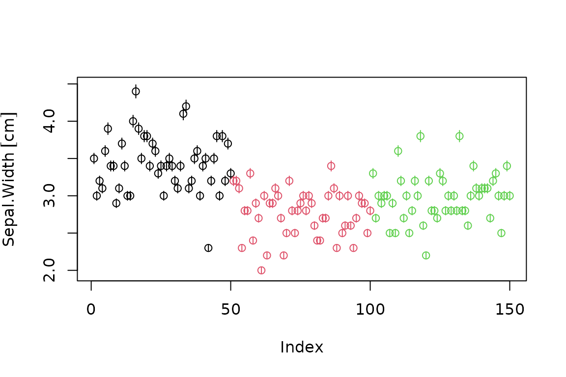
Quantities support R base scatterplots out of the box: errors are displayed as segments around each point and units are automatically added to the corresponding axis label.

Here is an example of a simple plot of a single quantity, where each value is automatically indexed in the x-axis:

# vector plots
with(iris.q, plot(Sepal.Width, col=Species))

X-Y scatterplots support units and errors in both axes:

# x-y plots
with(iris.q, plot(Sepal.Length, Sepal.Width, col=Species))
# dataframe plots
plot(iris.q[, c("Sepal.Length", "Sepal.Width")], col=iris.q$Species)

which are equivalent, and produce the same result, as the formula method:

plot(Sepal.Width ~ Sepal.Length, iris.q, col=Species)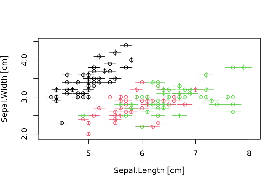

There is a fundamental limitation in R base for mixed quantities and non-quantities data due to S3 dispatch. It is possible, for instance, to plot quantities in the x-axis and numeric data in the y-axis:

plot(as.numeric(Sepal.Width) ~ Sepal.Length, iris.q, col=Species)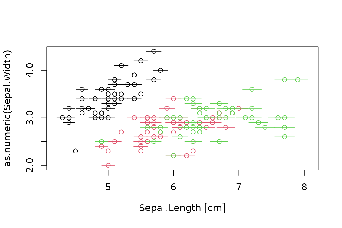

However, when the x-axis has numeric data, quantities methods will not be dispatched for the y-axis:

plot(Sepal.Width ~ as.numeric(Sepal.Length), iris.q, col=Species)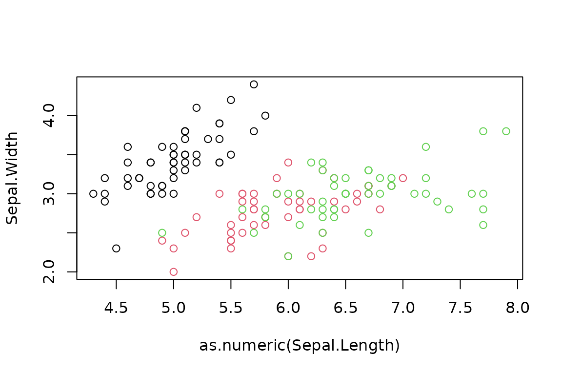

One way to overcome this limitation is to set unitless and errorless quantities in the x-axis:

plot(Sepal.Width ~ set_quantities(as.numeric(Sepal.Length), 1, 0), iris.q, col=Species)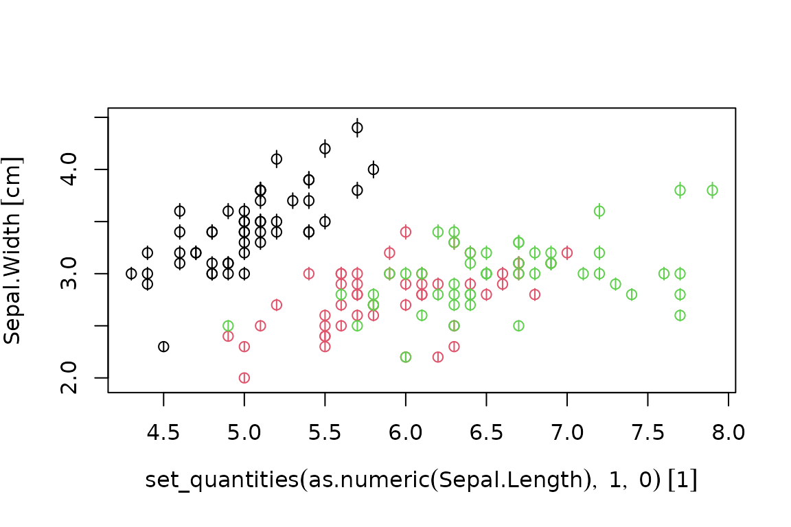

Tidyverse

The core tidyverse includes the following packages: ggplot2, dplyr, tidyr, readr, purrr, tibble, stringr and forcats. This section covers use cases for dplyr (everything except for pivoting and unpivoting), tidyr (for pivoting and unpivoting) and ggplot2 (for plotting).

library(dplyr); packageVersion("dplyr")
#> [1] '1.1.4'
library(tidyr); packageVersion("tidyr")
#> [1] '1.3.1'

Although not strictly necessary, we will convert the data frame to tibble format to enjoy the formatting provided by pillar.

iris.q <- as_tibble(iris.q)
head(iris.q)
#> # A tibble: 6 × 5
#>   Sepal.Length Sepal.Width Petal.Length Petal.Width Species
#>     (err) [cm]  (err) [cm]   (err) [cm]  (err) [cm] <fct>  
#> 1       5.1(1)     3.50(7)      1.40(3)    0.200(4) setosa 
#> 2       4.9(1)     3.00(6)      1.40(3)    0.200(4) setosa 
#> 3      4.70(9)     3.20(6)      1.30(3)    0.200(4) setosa 
#> 4      4.60(9)     3.10(6)      1.50(3)    0.200(4) setosa 
#> 5       5.0(1)     3.60(7)      1.40(3)    0.200(4) setosa 
#> 6       5.4(1)     3.90(8)      1.70(3)    0.400(8) setosa

Since dplyr 1.0.0, as we will see, there is enhanced support for custom S3 classes thanks to the new implementation based on vctrs >= 0.3.0. Packages units >= 0.6-7, errors >= 0.3.4 and quantities >= 0.1.5 add support for this approach.

Row Subsetting

The filter generic finds observations where conditions hold. The main difference with base subsetting is that, if a condition evaluates to NA for a certain row, it is dropped. As in the base case, another quantities object must be defined for the comparison:

iris.q %>%
  filter(Sepal.Length > set_quantities(75, mm)) %>%
  head()
#> # A tibble: 6 × 5
#>   Sepal.Length Sepal.Width Petal.Length Petal.Width Species  
#>     (err) [cm]  (err) [cm]   (err) [cm]  (err) [cm] <fct>    
#> 1       7.6(2)     3.00(6)       6.6(1)     2.10(4) virginica
#> 2       7.7(2)     3.80(8)       6.7(1)     2.20(4) virginica
#> 3       7.7(2)     2.60(5)       6.9(1)     2.30(5) virginica
#> 4       7.7(2)     2.80(6)       6.7(1)     2.00(4) virginica
#> 5       7.9(2)     3.80(8)       6.4(1)     2.00(4) virginica
#> 6       7.7(2)     3.00(6)       6.1(1)     2.30(5) virginica

There are also three scoped variants available (filter_all, filter_if, filter_at) and a subsetting function by row number called slice. All of them preserve quantities.

Row Ordering

The arrange generic sorts variables in a straightforward way, and it is compatible with quantities:

iris.q %>%
  arrange(Sepal.Length) %>%
  head()
#> # A tibble: 6 × 5
#>   Sepal.Length Sepal.Width Petal.Length Petal.Width Species
#>     (err) [cm]  (err) [cm]   (err) [cm]  (err) [cm] <fct>  
#> 1      4.30(9)     3.00(6)      1.10(2)    0.100(2) setosa 
#> 2      4.40(9)     2.90(6)      1.40(3)    0.200(4) setosa 
#> 3      4.40(9)     3.00(6)      1.30(3)    0.200(4) setosa 
#> 4      4.40(9)     3.20(6)      1.30(3)    0.200(4) setosa 
#> 5      4.50(9)     2.30(5)      1.30(3)    0.300(6) setosa 
#> 6      4.60(9)     3.10(6)      1.50(3)    0.200(4) setosa

The desc function can be applied to individual variables to arrange in descending order.

Column Transformation

There are two generics for column transformations: mutate modifies or adds new variables preserving the existing ones, while transmute drops the existing variables. The syntax is very similar to base functions transform and within, and equally compatible with quantities:

iris.q %>%
  transmute(
    Species = Species,
    Petal.Area = Petal.Length * Petal.Width,
    Sepal.Area = Sepal.Length * Sepal.Width
  ) %>%
  head()
#> # A tibble: 6 × 3
#>   Species   Petal.Area   Sepal.Area
#>   <fct>   (err) [cm^2] (err) [cm^2]
#> 1 setosa      0.280(8)      17.8(5)
#> 2 setosa      0.280(8)      14.7(4)
#> 3 setosa      0.260(7)      15.0(4)
#> 4 setosa      0.300(8)      14.3(4)
#> 5 setosa      0.280(8)      18.0(5)
#> 6 setosa       0.68(2)      21.1(6)

Row Aggregation

dplyr breaks down aggregation operations in two distinct parts: grouping (with group_by) and summarising (using summarise and others). Since dplyr >= 1.0.0, operations on aggregated data is now fully compatible with quantities and,compared to base methods, no fancy unlisting is required:

iris.q %>%
  group_by(Species) %>%
  summarise_all(mean)
#> # A tibble: 3 × 5
#>   Species    Sepal.Length Sepal.Width Petal.Length Petal.Width
#>   <fct>        (err) [cm]  (err) [cm]   (err) [cm]  (err) [cm]
#> 1 setosa           5.0(1)     3.43(7)      1.46(3)     0.25(1)
#> 2 versicolor       5.9(1)     2.77(6)      4.26(9)     1.33(3)
#> 3 virginica        6.6(1)     2.97(6)       5.6(1)     2.03(4)

Column Joining

Several verbs are provided for different types of joins, such as inner_join, left_join, right_join or full_join. Internally, they use the same grouping mechanism than summaries. Therefore, since dplyr >= 1.0.0, these are fully compatible with quantities too:

iris.q %>%
  left_join(data.frame(
    Height = set_quantities(c(55, 60, 45), cm, c(45, 30, 35)),
    Species = c("setosa", "virginica", "versicolor")
  )) %>%
  head()
#> Joining with `by = join_by(Species)`
#> # A tibble: 6 × 6
#>   Sepal.Length Sepal.Width Petal.Length Petal.Width Species     Height
#>     (err) [cm]  (err) [cm]   (err) [cm]  (err) [cm] <chr>   (err) [cm]
#> 1       5.1(1)     3.50(7)      1.40(3)    0.200(4) setosa      60(40)
#> 2       4.9(1)     3.00(6)      1.40(3)    0.200(4) setosa      60(40)
#> 3      4.70(9)     3.20(6)      1.30(3)    0.200(4) setosa      60(40)
#> 4      4.60(9)     3.10(6)      1.50(3)    0.200(4) setosa      60(40)
#> 5       5.0(1)     3.60(7)      1.40(3)    0.200(4) setosa      60(40)
#> 6       5.4(1)     3.90(8)      1.70(3)    0.400(8) setosa      60(40)

The only difference with base merge here is that dplyr does not reorder columns with respect to the left-hand side.

(Un)Pivoting

Finally, pivoting and unpivoting is handled by a separate package, tidyr. Historically, this was managed using the verbs spread (pivot) and gather (unpivot). These verbs, which are not compatible with quantities, are deprecated and no longer maintained.

Instead, there are new and more straightforward verbs for (un)pivoting data frames called pivot_wider (equivalent to spread) and pivot_longer (equivalent to gather). These verbs do make use of the new approach brought by vctrs and therefore are fully compatible with quantities.

Compared to base R, the unpivoting operation is substantially more straightforward. In the next example, we directly merge the four columns of interest into the value column, and the correspoding column names are gathered into the name column. Such a column is then separated into flower part (sepal, petal) and dim (length, height):

iris.q %>%
  pivot_longer(1:4) %>%
  separate(name, c("part", "dim")) %>%
  head()
#> # A tibble: 6 × 4
#>   Species part  dim         value
#>   <fct>   <chr> <chr>  (err) [cm]
#> 1 setosa  Sepal Length     5.1(1)
#> 2 setosa  Sepal Width     3.50(7)
#> 3 setosa  Petal Length    1.40(3)
#> 4 setosa  Petal Width    0.200(4)
#> 5 setosa  Sepal Length     4.9(1)
#> 6 setosa  Sepal Width     3.00(6)

In the following example, we first unpivot the original data set, then we assign quantities and try to pivot it to obtain iris.q back, and it just works:

iris %>%
  # first gather, with row numbers as row_id
  mutate(row_id = 1:n()) %>%
  pivot_longer(1:4) %>%
  # assign quantities
  mutate(value = set_quantities(value, cm, value * 0.05)) %>%
  # now spread and remove the row_id
  pivot_wider() %>%
  select(-row_id) %>%
  head()
#> # A tibble: 6 × 5
#>   Species Sepal.Length Sepal.Width Petal.Length Petal.Width
#>   <fct>     (err) [cm]  (err) [cm]   (err) [cm]  (err) [cm]
#> 1 setosa        5.1(3)      3.5(2)      1.40(7)     0.20(1)
#> 2 setosa        4.9(2)      3.0(1)      1.40(7)     0.20(1)
#> 3 setosa        4.7(2)      3.2(2)      1.30(6)     0.20(1)
#> 4 setosa        4.6(2)      3.1(2)      1.50(7)     0.20(1)
#> 5 setosa        5.0(2)      3.6(2)      1.40(7)     0.20(1)
#> 6 setosa        5.4(3)      3.9(2)      1.70(8)     0.40(2)

Plotting

library(ggplot2); packageVersion("ggplot2")
#> [1] '3.5.1'

Quantities packages provide ggplot2 elements to make scatterplots straightforward:

units provides automatic detection of units scale type, with optional conversion and customization via scale_x_units() and scale_y_units().
errors provides automatic placement of errorbars via geom_errors().
quantities provides a compatibility layer between them, so that conversions from scale_[x|y]_units affect errorbars too.

By default, units are automatically placed in the axes:

p0 <- ggplot(iris.q) + aes(Sepal.Length, Sepal.Width, color=Species) +
  geom_point()
p0
#> Warning: The `scale_name` argument of `continuous_scale()` is deprecated as of ggplot2
#> 3.5.0.
#> This warning is displayed once every 8 hours.
#> Call `lifecycle::last_lifecycle_warnings()` to see where this warning was
#> generated.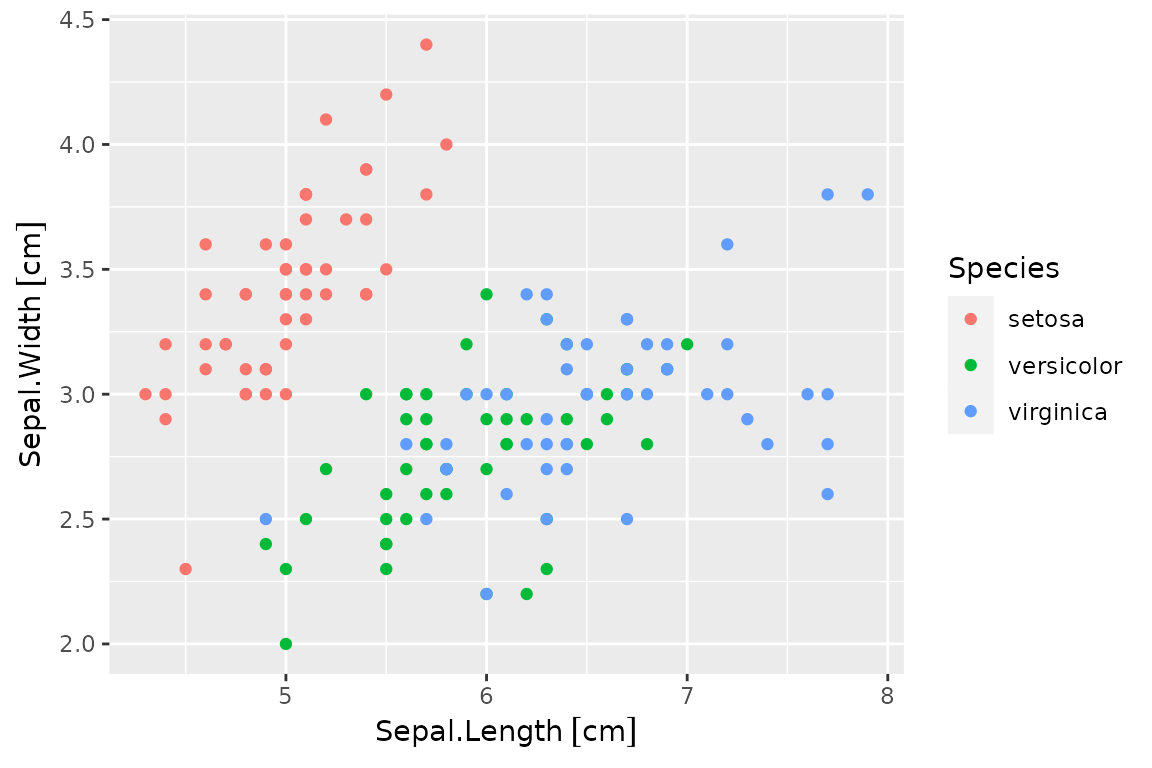

And errobars can be requested via geom_errors():

p0 + geom_errors()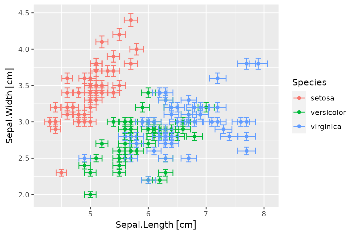

Errors may be dropped from any axis:

p0 + geom_errors(aes(x=drop_errors(Sepal.Length)))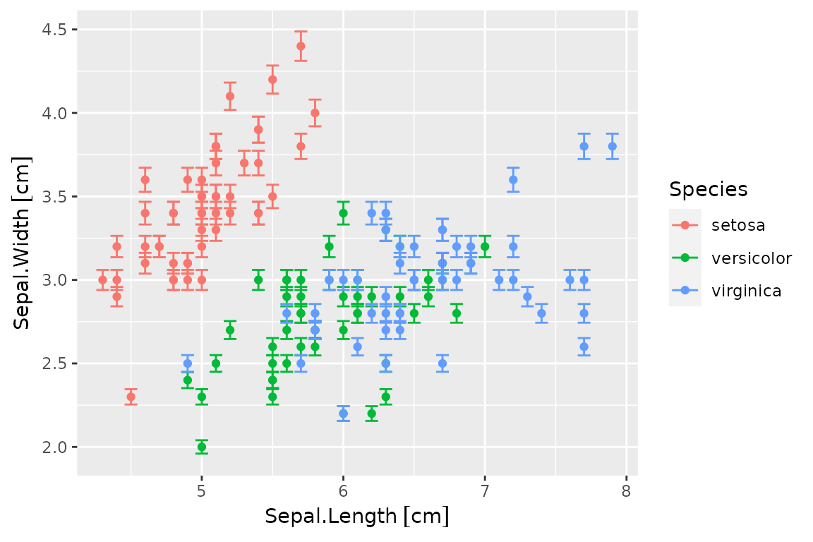

And units can be converted for display:

p0 + geom_errors() + scale_x_units(unit="mm") + scale_y_units(unit="m")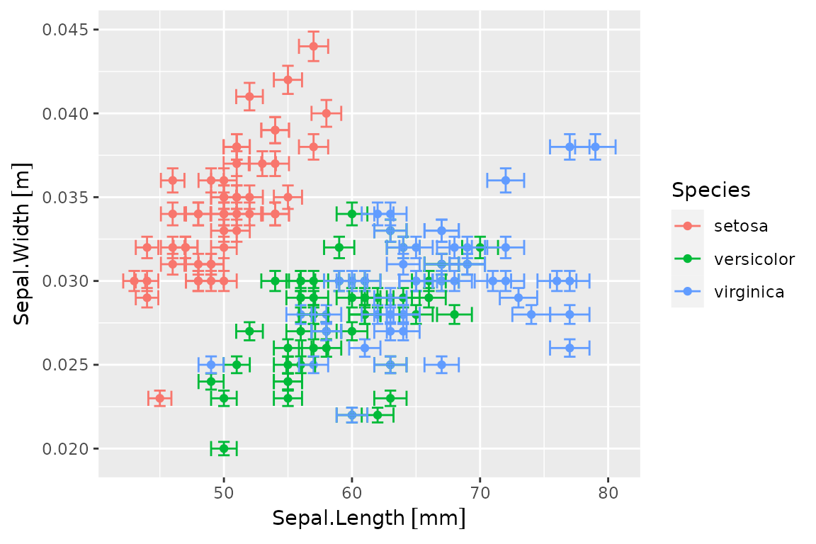

Summary

R base works smoothly with quantities in most cases. The only shortcoming is that some care must be applied to aggregations. In particular, simplification must be explicitly disabled (simplify=FALSE), and such a simplification (i.e., converting lists to vectors of quantities) must be applied manually while avoiding unlist.

Since dplyr 1.0.0 and tidyr 1.1.0 (for units >= 0.6-7, errors >= 0.3.4 and quantities >= 0.1.5), the new vctrs-based approach brings us full compatibility with quantities for all the operations considered in this document, including grouped operations, joining and pivoting, which did not work for previous versions.

Both R base and ggplot2 plots work out of the box, although the latter provides much more flexibility and can be used independently of the tidyverse.

A Note on `data.table`

The data.table package is another popular data tools, which provides a high-performance version of base R’s data.frame with syntax and feature enhancements for ease of use, convenience and programming speed.

Long story short, we have not included a section on data.table because currently (v1.11.4) it does not work well with vectorised attributes. The underlying problem is similar to dplyr’s issue, but unfortunately it affects more operations, including row subsetting and ordering. Only column transformation seems to work, and other operations generate corrupted objects.

We have found that defining quantities columns as lists (where each element consists of a single value, with unit and uncertainty) may be a workaround, but this probably would be a serious performance penalty for a package that is typically chosen for speed reasons.

Iñaki Ucar

2024-07-29

Introduction

R Base

Row Subsetting

Row Ordering

Column Transformation

Row Aggregation

Column Joining

(Un)Pivoting

Plotting

Tidyverse

Row Subsetting

Row Ordering

Column Transformation

Row Aggregation

Column Joining

(Un)Pivoting

Plotting

Summary

A Note on `data.table`

A Guide to Working with Quantities

Iñaki Ucar

2024-07-29

Introduction

R Base

Row Subsetting

Row Ordering

Column Transformation

Row Aggregation

Column Joining

(Un)Pivoting

Plotting

Tidyverse

Row Subsetting

Row Ordering

Column Transformation

Row Aggregation

Column Joining

(Un)Pivoting

Plotting

Summary

A Note on data.table

A Note on `data.table`